NEQNET: Non-equilibrium Phenomena

Cosmology, turbulence, markets, non-equilibrium QFT and much more. No nonsense, just science

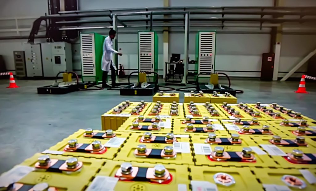
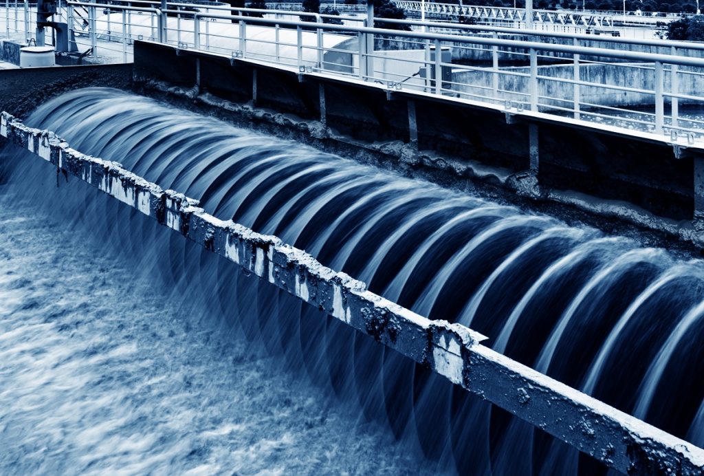
381. M2 branes and Chern-Simons theories

John Davey is a PhD student of Amihay Hanany at Physics Department of Imperial College, London. Dmitry.

Recently Chern-Simons theories have attracted much attention as they are thought to describe the world volume theory of the elusive M2 brane. In this short article I will attempt to outline some of the recent developments in this field and describe how brane tilings can be used to find and investigate a large class of these theories.

The recent interest in the topic of M2 branes was triggered by the discovery of highly supersymmetric Chern-Simons theories. Any theory that describes the world volume physics of an M2 brane should be maximally supersymmetric in 3 dimensions. Such a theory should therefore admit N=8 SUSY. Previously, it was thought that Chern-Simons theories in three dimensions can have at most N=3 SUSY, however Bagger and Lambert [1] recently found a Chern-Simons theory which admits the full N=8 symmetry and fits perfectly as a theory for M2 branes in flat space. Aharony, Bergman, Jafferis, and Maldacena later found the the world volume theory of a stack M2 branes transverse to a geometry [2].

A 2+1 dimensional Chern-Simons (CS) theory is a quantum field theory that has a non-dynamical gauge field . The action for such a theory has the form

Where we take to be a non-abelian gauge field transforming in the adjoint representation of the gauge group U(N).

In order for the theory to make sense, it must be well behaved under gauge transformations. While it is relatively easy to show invariance in the abelian case, the non-abelian case is a little more subtle. In this case

Where N is a integer related to the winding number of the gauge transformation performed. When quantizing the theory using Feynman’s path integral formalism, we insist upon being gauge invariant. This leads to the condition that . This integer k is called the Chern-Simons level for the gauge field . Typically every gauge group in the Chern-Simons theory has a level associated to it.

The Chern-Simons theory above is not at all supersymmetric. However it is possible to make the gauge field a component of an N=2 vector multiplet. Doing this necessarily introduces two scalar fields (one of them auxiliary) and a 2-component dirac spinor to the theory. Supersymmetry invariance naturally enhances the action to include many new terms, including the possibility of superpotential terms. Exactly which superpotential terms, and Chern-Simons levels we pick affects how much more additional supersymmetry the theory has. By carefully consideration of these factors, it is possible to find a theory that can admit the full N=8 SUSY (16 supercharges).

For certain special Chern-Simons theories we can pictorally represent the Lagrangian by using a directed graph called a quiver diagram. These theories are called quiver gauge theories. Each node of the quiver corresponds to a gauge group and each edge corresponds to a chiral field. Each chiral field transforms under a bi-fundamental representation of the two gauge groups that the edge connects. To define the quiver gauge theory’s lagrangian, superpotential data must also be supplied. In this discussion we shall insist that each field should appear exactly twice in the superpotential – once in a positive and once in a negative term. This is known as the toric condition. It should be noted that, due to gauge invariance, each superpotential term corresponds to a closed loop in the quiver, although the converse is not always true. To completely specify the theory living in the world volume of a stack of M2 branes, we must also specify Chern-Simons levels for all of the gauge groups in the theory.

A brane tiling can be viewed as an extension of a quiver to include superpotential data. The tiling is a bi-partite graph that lives on , or alternatively one can view it as forming a tiling of the plane. The tiling’s dual graph is the periodic quiver and so the tiling’s faces correspond to gauge groups and its edges correspond to chiral bi-fundamental fields. A given term in the superpotential is composed of all of the fields (edges) that the corresponding node connects to. As the tiling is bi-partite we can colour its nodes, say, black and white with different coloured nodes corresponding to superpotential terms of different signs. The tiling’s superpotential then naturally satisfies the toric condition as each edge connects precisely one white and one black node. As is mentioned above, Chern-Simons levels must also be specified to fully define the theory. Faces in the tiling are given integers equal to these Chern-Simons levels.

Once a brane tiling and a set of Chern-Simons terms are chosen then it is interesting to analyse the Moduli Space of Vacua of the theory.  For CS theories with superpotentials satisfying the toric condition, this space is generically a toric Calabi-Yau 4-fold.  The first and in some ways most simple object we look at is the space of vacua when only the superpotential’s F-terms are taken into account. This space is known as the Master Space of the theory and can be given by the quotient where can be regarded as a charge matrix associated with the F-terms. The space is a space of special liner combinations of fields called perfect matchings. A perfect matching is a collection of fields such that each term in the superpotential contains exactly one of these fields. These perfect matchings can be found easily from the tiling [3] and , which encodes the relationships between these perfect matchings, is also very easy to find.  The columns of  correspond to perfect matchings and rows of  correspond to charges.

It is also possible to take into account the D-term conditions. The moduli space of vacua, taking into account both F-terms as well as D-terms is called the mesonic moduli space and can be identified with the space transverse to an M2-brane in M-theory.  Rows of the charge matrix correspond to baryonic symmetries of the theory and tell us how perfect matchings (corresponding to columns) are charged under these symmetries. The computation of   is straightforward and is described in [3].  It turns out that the total number of charges (from both and ) is equal to which means that the (complex) dimension of the mesonic moduli space is equal to 4. This is expected as there should be 8 real (or 4 complex) dimensions transverse to an M2 brane in 11 dimensional M-theory.

The mesonic moduli space, being a toric Calabi-Yau 4-fold, can be specified by a convex collection of lattice points in called a toric diagram, which is a kind of fingerprint for the manifold. This toric diagram can be found directly from the and matrices that define the theory’s mesonic moduli space. The total charge matrix can constructed by gluing together the two charge matrices:

The kernel of this total charge matrix contains the toric data of the CY 4 of interest. Specifically, a collection of 4-vectors are generated which form a convex zonotope in . We should note that the toric points live in a 3-dimensional hypersurface in this 4-dimensional space, which is a manifestation of the Calabi-Yau condition on the mesonic moduli space. This collection of toric points defines the aforementioned toric diagram. The process of finding this toric data for a given Chern-Simons theory is known as the forward algorithm and is a very efficient way of finding large numbers of Chern-Simons theories that live on M2 branes. Given a tiling and a set of Chern-Simons levels, we can easily compute details of the mesonic moduli and so find out which M2 brane geometry the Chern-Simons theory corresponds to. As a special case, we find the well known ABJM theory [2].

One interesting phenomena worthwhile mentioning is that of toric duality. This is when two different CS theories, corresponding to two different tilings with different CS levels have the same mesonic moduli space and so describe the same M2 brane physics. This phenomena is well known and is called toric duality. In Phases of M2-brane Theories [3], these dualities are tested by comparing both the spectrum of gauge invariant operators and also scaling dimensions.

References:

[1]  J. Bagger and N. Lambert, arXiv:0712.3738 [hep-th].

[2] O. Aharony, O. Bergman, D. L. Ja eris and J. Maldacena, arXiv:0806.1218 [hep-th].

[3] J. Davey, A. Hanany, N. Mekareeya and G. Torri arXiv:0903.3234 [hep-th].

380. Lightest exoplanet found: video of the day

… as announced on Apr 21. Discovered planet is only about twice as massive the Earth.

379. Thermonuclear fusion: list of posts

Before proceeding to the discussion of hydrodynamic instabilities in plasma, let me list for further reference all the posts I wrote so far about thermonuclear fusion and thermonuclear reactors:

1. Thermonuclear fusion: some basic facts about thermonuclear reactions, where I start explaining why such phenomenon as thermonuclear fusion can even take place in Nature I also briefly discuss the issue of Coulomb barrier and two possible strategies to overcome it.

2. Thermonuclear fusion. Coulomb barrier and reaction rates, where several important fusion reactions are listed and reaction rates (defined by the Gamov exponent) are estimated by means of quasiclassical approximation.

3. Thermonuclear fusion. Nuclear reaction rates – second part, where I estimate reaction rate from the naive kinetic theory and find its dependence on temperature.

4. Introduction into thermonuclear reactors, where the criterion for thermonuclear reactions to be self-sustained is represented and we discuss two classes of reactors based on the type of plasma confinement used. After that post thermonuclear reactors with magnetic confinement will be almost completely forgotten

5. Thermonuclear reactors. Inertial confinement, where we calculate reaction rate in thermonuclear reactors with inertial confinement.

6. Thermonuclear reactors. More on inertial confinement, devoted to discussion of a couple of important parameters that characterize thermonuclear reactors with inertial confinement.

7. Inertial confinement – using lasers for compression, where it is explaned how inertial confinement works and why it has any meaning to use lasers for compressing the plasma and ignition.

8. Inertial confinement: more on interaction of laser emission with matter, where important mechanisms of laser/matter (material of the fuel capsule) interaction and scenarios of behavior of matter in the fuel capsule after ignition are discussed.

378. Sounds of Jupiter: video (or better say – audio?) of the day

Damn if it does not sound like Stanley Kubrick’s “2001: Space odyssey” Did he actually know? Although these particular sounds were recorded in 1988, I bet people have heard them back in 1950s-60s, and Clarke should have told Kubrick about them.

377. Temporal and spatial dependence of quantum entanglement

Shih-Yuin Lin is a professor at Physics Division, National Center for Theoretical Sciences, Taiwan. Dmitry.

In textbooks, quantum entanglement are often introduced to readers with the simplest case: in an isolated system with two parties or subsystems, if a quantum states can be factorized into a product of the quantum states for each subsystem,

then it is called a separable state, otherwise it is entangled. For a separable state, the quantum state of one party will not be affected by any local measurement on the other, but for an entangled state, it will.

Usually in their examples there is no indication of the positions of the two (or more) subsystems or quantum objects. The quantum objects such as two spins or atoms can be located very far away from each other, e.g. the A-party is at Helsinki Institute of Physics while the B-party is at some planet in Andromeda Galaxy. They can also be located at the same point in space, anyway, with the two parties being different degrees of freedom, provided that it is possible to perform “local” operations on each party without disturbing the other (in other words, those operations on different parties commute).

As a physical property, entanglement is independent of the representation of each party. But entanglement of a quantum system does depend on partition: one can always perform a “global” canonical transformation or a mixing on variables of all parties to make an entangled state in the old variables separable in the new variables. We don?t need to worry about this, however, because when we are talking about quantum entanglement between two objects, we have actually assigned some preferred set of dynamical variables which are going to be measured locally — according to the apparatus in our hands or in our minds. Physical considerations will determine which way of partition or which set of dynamical variables is natural.

Quantum entanglement in open quantum systems

In a more realistic situation, the system we are looking at will be inevitably coupled with the environment, which could be as innocent as a mediating quantum field in free space or in medium at some temperature. Then the dynamics of the system should be described by the reduced quantum state (the reduced density matrix, RDM) for the system, which is obtained by integrating (or averaging) out the degrees of freedom of the environment in the density matrix of the combined system. The RDM of the system is in general a mixed state, which is a probabilistic sum of the density matrices of pure quantum states of the system. It carries both quantum and statistical natures.

What is quantum entanglement for a mixed state? For a bipartite system, a mixed state is said to be entangled if it CANNOT be written as a convex sum of direct products of the density matrices of each party,

(which can be modeled by local hidden-variable theories). Unfortunately this definition of quantum entanglement is not constructive. This makes the construction of well-defined degrees of entanglement for mixed states very hard and rarely successful — So far the well-defined ones exist only for systems with (a) two 2-level atoms, and (b) two Gaussian states!

This is actually a good excuse for us — to get a concrete result on entanglement dynamics, we have to design our thought experiment by employing one of these two categories, both are simple enough. Thus in [1] and [2] we employ the latter: Gaussian states in the Unruh-DeWitt (UD) detector theory.

The UD detector is a point-like object with its internal degree of freedom linearly coupled to a quantum field while its trajectory is put in by hand [1]. It is an analogy for an atom in EM field, rather than a real, macroscopic detector in laboratory. By choosing the internal degree of freedom of the detector as a harmonic oscillator* and the quantum field as a massless scalar field in Minkowski space, the combined system is linear, and we are able to solve the full dynamics of the detector-field system.

*Historically the interacting action of the Unruh-DeWitt detector theory was applied to demonstrate the Unruh effect in time-dependent perturbation theory by Bill Unruh (1976) and Bryce DeWitt (1979), without specifying the structure of the free detector. The present form with harmonic oscillators as the internal degrees of freedom is employed by several authors later for simplicity.

Temporal dependence of entanglement

In open quantum systems, the initial state of interest, e.g., a direct product of the quantum state for the system and the one for the environment, is usually not an eigenstate of the combined system. So the quantum state for the detectors or atoms as well as the one for the field (our environment) will all evolve in time (non-equilibrium phenomena!), which makes quantum entanglement between the detectors or atoms time-varying.

There are all kinds of entanglement dynamics in open quantum systems, some are not quite intuitive due to the somewhat curious definition of quantum entanglement for mixed states. For example, two initially entangled objects immersed in the environment can be completely disentangled in finite time. This is called the “sudden death” of entanglement.

Entanglement dynamics of two 2-level atoms in two independent cavities. C(t) is the “concurrence”, which is a measure of entanglement of these two atoms, and a is a parameter of the initial state. Different values of a gives different behaviors. From Yu, Eberly, PRL 93, 140404 (2004).

In contrast, two initially separated objects in the environment can be entangled after a finite time. This is called the entanglement creation or generation.

Entanglement creation of two spins coupled with a spin chain. From Lai, Hung, Mou, Chen, PRB77, 205419 (2008)

In some cases entanglement can revive after sudden death, or insists until late times and becomes residual entanglement.

Entanglement dynamics of two harmonic oscillators located at the same point in a quantum field. E_N is the logarithm negativity, which is a degree of quantum entanglement. From Paz and Roncaglia, PRL100, 220401 (2008).

Spatial dependence of entanglement

Moreover, the properties of the environment will enter the entanglement dynamics of the system through the coupling. This is why the Unruh-DeWitt detectors are called ?detectors?: Their responses reveal the characteristics of the environment. For localized quantum objects, one of the consequences from coupling with the environment is the dependence of entanglement dynamics on the positions of them.

For two localized detectors and coupled with a common massless quantum field in free space, the back-reaction of the detector to the field will propagate out in light speed (because the field is massless) then drive the other detector , whose response will again back-act to the field and propagate back to drive the detector . The additional response of the detector to these echoes will then propagate out, and so forth. These generate the mutual influences between the detectors, which depend on how the information propagates in the environment very much. They cannot be faster than light, so they are explicitly causal.

Two detectors L and R are at rest and separated at a distance d in Minkowski space. The coupling between the detectors and the field is switched on at t=0.

Besides, in quantum fields there exist non-vanishing correlations between vacuum fluctuations of the fields at spacelike separated events. While these correlations are non-local in some sense, they still cannot be used for sending signal to violate causality.

Of course, in more complicated situations with more complicated environment such as spin chains or cavities with strange boundaries, or with more nontrivial motions of the detectors such as those in acceleration or sitting around a black hole [2], or with nonlinear interactions in the detectors and/or the environment, the response of the detectors or atoms will be more complicated. But as far as we know even in the simplest models the full dynamics were hardly well-understood by physicists. Thus in [1] we start with the simplest case we can imagine: We consider a model with two Unruh-DeWitt detectors, both at rest and separated at a distance d, coupled with a common massless scalar field at zero temperature in Minkowski coordinate.

We find that the dynamics of entanglement in our model depend on the spatial separation between the detectors in a non-trivial way. Both the two factors mentioned above, (1) phase difference of the quantum noise experienced locally by each detector, and (2) interference of the retarded mutual influences, can lead to the spatial dependence.

For an initially entangled pair of detectors, when one gets inside the light cone of the other (started from the other detector at the initial moment of switching on the interaction), certain interference pattern in d develops. At distances where the interference is constructive the disentanglement times are longer than those at other distances. This behavior is more distinct when the mutual influences are negligible; It is mainly coming from the factor (1).

Evolution of quantum entanglement of an initially entangled pair of detectors sitting at rest in vacuum state of a massless scalar field in Minkowski coordinate. E_N is the logarithm negativity, which is a degree of quantum entanglement. For fixed d, as t increases, E_N is falling so the detectors are disentangling. E_N,rel is roughly the relative value of the E_N at finite d to the E_N at spatial infinity on the same time slice. You can see there are some interference patterns in d inside the light cone and in t outside the light cone.

On the other hand, for an initially separable state, the mutual influences (factor (2)) can generate entanglement from nothing if the spatial separation is sufficiently small.

We noticed that the entanglement is created deeply in the light cone, meaning that before the entanglement is generated the two detectors have had conversations back and forth for several rounds to synchronize their steps and build up the coherence.

Some authors suggested that entanglement can be generated by the environment even when one atom is still outside the light cone of the other. But in our simple model, we did not see any evidence of entanglement creation outside the light cone, though for the initially entangled states, the phase difference of quantum noise of the environment does produce interesting entanglement dynamics between the detectors located far apart: At some moments the larger the separation the weaker the entanglement, but at other moments, the stronger the entanglement. Such a behavior is again caused by factor (1).

Outlook

As pointed out by Erwin Schr?dinger, quantum entanglement is ?not ONE but THE characteristic trait of quantum mechanics?, so it is THE resource in quantum information science (including, e.g., quantum imaging, quantum teleportation, quantum communication, and so on) and plays the most important role in understanding the foundation of quantum physics. Nevertheless, quantum entanglement is more delicate than correlations and coherences in open quantum systems: It can give you surprises even in the simplest models. Today we are still in a status of gaining more and more experiences and intuitions on entanglement dynamics in different non-equilibrium systems. We hope we can handle and manipulate it in the near future.

References

[1] Shih-Yuin Lin and Bei Lok Hu, Phys. Rev. D 79, 085020 (2009) [arXiv: 0812.4391].
[2] Shih-Yuin Lin, Chung-Hsien Chou, and Bei Lok Hu, Phys. Rev. D 78, 125025 (2008) [arXiv:0803.3995].
[3] E. Calzetta, B.-L. Hu, Non-equilibrium quantum field theory.
[4] F. Benatti, Irreversible quantum dynamics.

Did not find what you were looking for? Try

Copyright 2008-2009. "NEQNET: Non-equilibrium Phenomena" by Dmitry Podolsky. All rights reserved.