NEQNET: Non-equilibrium Phenomena

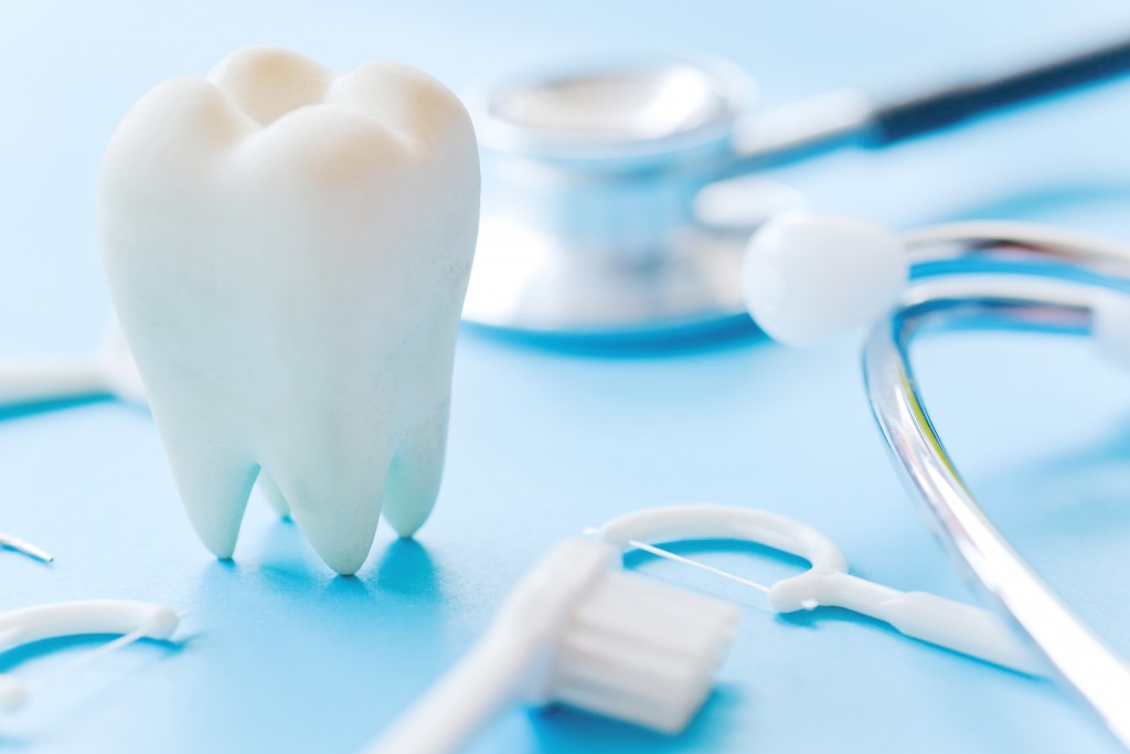
41. Peter Woit: What will you do if string theory is wrong?

Posted by Dmitry

at May 9, 2008

Sorry for entering into dicussions irrelevant for physics, but Peter Woit’s post really touched something deep inside of me :-)

As I understand, the Peter Woit’s logic and the logic of people entered discussion on his blog mostly works as follows:

a) string theory is WRONG

b) if so, all string theorists should be immediately fired

(Peter Shor regretfully replies: “No, they are on a tenure, you cannot fire them so easily”.)

I have an impression that whether string theory is right or wrong really depends on the question you ask, and it does not look like Peter asked any physical question.

If you ask “Does landscape has anything to do with objective reality?”, then the answer could be “no” (or could be well a sounding “yes”, if we learn how to contruct observables on the landscape and measure them).

If you ask whether string theory has anything to do with strongly coupled YM, confinement of quarks or, say, 3D Ising model (the same universality class as most 2 order phase transitions in Nature), then the answer should be already known to you.

I think, if the landscapism will eventually die out, string theorists will find what to do, since the class of problems in Nature requiring string theory for their solution is very far from being empty.

Cheers

P.S. I have to confess (although it is painful) - about 5 years ago I was mostly reading Peter Woit’s blog, wanted to debunk string theory and was really embarassed by Lubos Motl’s rants on Woit :-) But sooner or later any person who is reading physics related blog starts trying to figure out what is the physical content of the post, what is the information it contains, since rants are rants, emotions are emotions, but we are really interested in CONTENT, aren’t we? As a result, nowadays the situation is the opposite compared to what was 5 years ago - I visit Peter’s blog really rarely and read Lubos’ rants much more often. Although I am very unhappy with the fact that Lubos started to write so much about physics unrelated things :-)

My reply to Peter

Peter

If I misitepreted your or Peter Shor’s words, I apologize. Nevertheless, your post left me with a particular impression (and I have to confess that it did not dissolve), and that was the reason why I wrote what I wrote.

(also - about 3D Ising, since there was a question about it)

For 2D Ising, there are two equivalent formulations of the theory: in terms of spin variables $\sigma$ and in terms of disorder variables $\mu$ (the ends of dislocation lines). Although $\sigma$ and $\mu$ satisfy rather complicated equations, their product satisfies linear equation; that fact allowed Onsager to find exact solution of the 2D Ising model.

For 3D Ising dislocation lines become dislocation surfaces, boundary of such surface is the variable on which disorder variable $\mu$ depends. One hope to find simple equations describing 3D Ising is to construct product of $\mu(C)$ and $\prod_i\sigma (x_i)$ where x_i are points close to the loop . Initial hope was that such a loop together with “spin” variables - vectors normal to loop and connecting it with points x_i - is NSR string, and the equation describing its dynamics is linear in the space of loops.

One person who tried to pursue this program was Polyakov. As far as I know, he got stuck since it was hard to write equations in loop space for renormalized variables.

Rate this:

2.5

These icons link to social bookmarking sites where readers can share and discover new web pages.

Various

51. Planck 2008: day 4 - Soft wall AdS/QCD

19. Disorder on the landscape: non-technical intro

47. Planck 2008: First and second days

23. Eye on ArXiv: 21 Apr 2008 - SUSY/non-SUSY duality

40. Inflation: field-theoretic description (Inflationary perturbations 4)

Posted by Dmitry

at May 9, 2008

This is the next post in the series based on my lectures on cosmological perturbations. Last time I discussed how inflation can be described only in terms of effective equation of state (with negative pressure). Today I am going to show how this equation of state can be realized at the quasi-classical level of QFT.

In order to describe the physics of inflation, a QFT model should have a distinctive feature: its hydrodynamic modes (i.e., such modes that their relaxation time goes to infinity while the wavelength goes to infinity) have to be described by the effective equation of state $p\approx-\rho$ . As a simple working example, let us consider a self-interacting scalar field $\varphi$ with potential $V(\varphi)$ ; at the level of phenomenology it can be a fundamental or a composite field (condensate of some kind).

The energy density stored in the hydrodynamic modes of \varphi is given by

$\rho=\frac{1}{2}(\dot{\varphi})^{2}+V(\phi),$ (1)

while the corresponding pressure is

$p=\frac{1}{2}(\dot{\varphi})^{2}-V(\phi).$ (2)

The realization of the de Sitter stage is possible if the kinetic energy of the scalar field is negligible compared to its potential energy. More precisely, expansion of the Universe will accelerate if

$\ddot{\varphi}\ll H\dot{\varphi},$ $\dot{\varphi}\ll H\varphi.$ (3)

Indeed, as follows from the Eqs. (1) and (2), $\rho\approx V(\varphi)$ and $p\approx-V(\phi)\approx-\rho$ in this case, so the Universe is de Sitter-like.

Dynamics of inflationary stage is the determined by the equation of motion for the scalar field

$\ddot{\varphi}+3H\dot{\varphi}+\frac{\partial V}{\partial\varphi}=0,$ (4)

where the friction term is defined by the Friedmann equation

$H^{2}=\frac{8\pi}{3M_{P}^{2}}\left(\frac{1}{2}(\dot{\varphi})^{2}+V(\varphi)\right).$ (5)

When the slow roll conditions (3) are valid, Hubble friction in the Eq. (5) dominates over the kinetic term and scalar field starts to slowly roll down towards the minimum of its potential. In this regime, one effectively has

$\frac{8\pi}{M_{P}^{2}}V(\varphi)\frac{d\varphi}{dN}=-\frac{\partial V}{\partial\varphi}$ (6)

(where is again the number of e-folds) with the solution

$N(\varphi)=\frac{M_{P}^{2}}{8\pi}\int_{\varphi}^{\varphi_{{\rm max}}}\frac{V(\phi)d\varphi}{\partial V/\partial\varphi},$

determining the number of e-folds of accelerated expansion $a(N)=a_{i}e^{N}$ as a function of $\varphi$ (please note that the number of e-folds turns out to be a more appropriate variable than the physical time during accelerated expansion stage; there is a deep physics in this statement, as we will see later when will discuss stochastic approach to eternal inflation). De Sitter stage can start at some

$\varphi_{{\rm max}}\lesssim\varphi_{P}$

such that $V(\varphi_{P})\sim M_{P}^{4}$ and continue until the conditions (3) break down at $\varphi=\varphi_{{\rm SR}}.$ The value of the Hubble parameter

$H\sim\frac{\sqrt{V(\varphi)}}{M_{P}^{2}}$

will slowly ( $|\dot{H}|\ll H^{2}$ ) decrease from $H_{i}=H(\varphi_{{\rm max}})$ to $H_{f}=H(\varphi_{{\rm SR}})$ , while the value of scale factor will quasiexponentially grow.

Let us show what happens explicitly taking the simplest possible model with potential

$V(\varphi)=\frac{1}{2}m^{2}\varphi^{2}$ .

Slow roll conditions (3) are satisfied when

$M_{P}\lesssim\varphi\lesssim\frac{M_{P}^{2}}{m},$

i.e., in the very wide range of possible values of $\varphi$ if $m\ll M_{P}$ . From the Eq. (6) we find

$\varphi(t)\approx\varphi_{{\rm max}}-\frac{mM_{P}}{\sqrt{12\pi}}(t-t_{i}).$

Therefore, the Hubble parameter decreases quadratically with time, while the scale factor grows as

$a(t)=a_{0}e^{\int Hdt}=a_{f}e^{-\frac{m^{2}}{6}(t-t_{f})^{2}},$

where $a_{f}$ is its value in the end of inflation. The overall length of the de Sitter stage is given by

$\delta t=t_{f}-t_{i}\approx\sqrt{12\pi}\frac{\varphi_{{\rm max}}}{mM_{P}}\lesssim2\sqrt{6\pi}\frac{M_{P}}{m^{2}},$

while the total number of e-folds accumulated during inflation is

$N\lesssim\exp\left(\frac{M_{P}^{2}}{m^{2}}\right)\sim\exp\left(10^{10}\right),$

where we took $m=10^{-5}\, M_{P}$ consistent with COBE normalization. As we see, the overall de Sitter stage could be extremely long, and the the size of homogeneous isotropic region by many orders of magnitude may exceed the present horizon size. Only last 60 or so e-folds of inflation give rise to the structure of the gravitational potential seen at near-horizon scale in the present universe.

The last thing remained to be explained in this Section is the Hamilton-Jacobi formalism for inflation. Often, it is more convenient to represent the Hubble parameter H=H(t) as a function of field $\varphi$ itself (of course, this can be done only if the field $\varphi$ changes monothonically with time). Second order differential equation (4) is equivalent to a pair of equations for the field and the Hubble parameter

$\dot{\varphi}=-\frac{M_{P}^{2}}{4\pi}H'(\varphi),$

$(H'(\varphi))^{2}-\frac{12\pi}{M_{P}^{2}}H^{2}(\phi)=-\frac{32\pi^{2}}{m_{P}^{2}}V(\varphi).$ (7)

The Eq. (7) is known as the Hamilton-Jacobi equation for inflation. Defining the slow roll parameter

$\epsilon=\frac{M_{P}^{2}}{4\pi}\left(\frac{H'}{H}\right)^{2},$

one can rewrite it as

$H^{2}(\varphi)\left(1-\frac{1}{3}\epsilon(\varphi)\right)=\frac{8\pi}{3M_{P}^{2}}V(\varphi).$

The meaning for the slow roll parameter $\epsilon$ is clear from the Friedmann equation $\frac{\ddot{a}}{a}=H^{2}(1-\epsilon)$ - it shows how rapidly effective cosmological constant changes with time. The reason why we mention the Gamilton-Jacobi equation here is that inflationary observables are typically represented as functions of slow roll parameter(s) and the Hubble scale at a given scale, not at a given time.