NEQNET: Non-equilibrium Phenomena

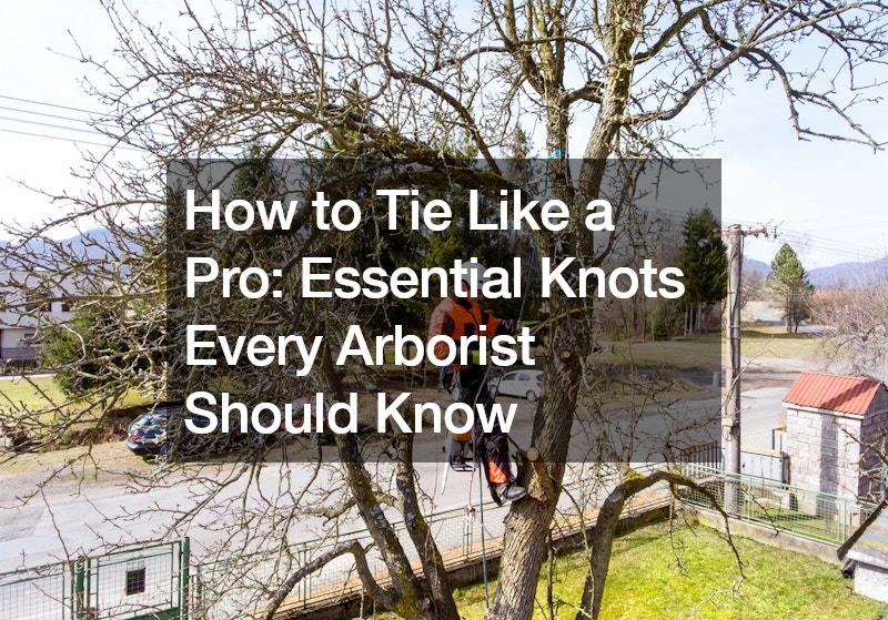
59. Eye on Arxiv: Quantum corrections to eta/s

Posted by Dmitry

at June 16, 2008

I decided to turn the de Sitter discussion off for a moment, it would be more appropriate to return to it after the paper is ready anyway :-) Hopefully, it will not take too much time for you to see it in ArXives.

Today I want instead to briefly discuss the paper “Quantum corrections to eta/s” by Myers et al.

As many of you are well aware of, in principle, AdS/CFT correspondence allows to understand (in the very first, rough, approximation) the non-equilibrium properties of the quark-gluon plasma. When I mention the word “non-equilibrium”, I actually do not mean dynamical properties of the plasma far away from the thermal equilibrium, but the regime where linear response analysis can be actually applied.

Although applying linear response to the strongly coupled QG plasma naively does not sound very physical, the nature turns out to work in such a way that very soon after the collision of two heavy nuclei (Au-Au, for example) dynamical equilibrium is reached in the sense that effective equation of state in the QG plasma is well settled down towards its equilibrium value. Although the real thermal equilibrium is very far from being achieved, the QG plasma is in the state which can be called “prethermalization”. In practice, prethermalization means that only UV part of the overall spectrum is relatively far from the thermal one, but we do not care about it much since IR low energy part interesting for us is well under control (for example, spectrum is power law like in turbulence or exsibits thermal behavior with some effective temperature $T_{\rm eff}$ , which is a slowly varying function of scale).

Anyway… in the “prethermalization” state one can apply linear response to understand behavior of non-equilibrium QFT correlators. This behavior is very far from being trivial because a) we discuss the state with very large occupation numbers and b) theory is effectively at strong coupling (we are talking about length scales $\gg\Lambda^{-1}_{\rm QCD}$ ).

The latter issue however can be treated by means of AdS/CFT; namely, we map strongly coupled QG plasma to gravity degrees of freedom propagating on the AdS background. The fact that we are dealing with conformal N=4 SYM instead of confining YM without any SUSY and number of colors equal 3 somehow does not bother us much because:

1) plasma is at large temperature, where scaling behavior effectively looks similar to CFT one
2) well, 1/N_c corrections are actually important but let us forget about them for a moment and see how far we will be able to advance :-)

Applying AdS/CFT immediately gives rise to a very interesting result: so called shear viscosity bound. Namely, as it turns out, for any gauge theories with an Einstein gravity dual in the limit of a
large number of colours and large t Hooft coupling $\lambda=g^2{}N_c\to\infty$

$\eta/s=\frac{1}{4\pi}$ (1)

and this result is claimed to be universal and even the lowest possible value of the shear viscosity in Nature (liquid He for example has larger shear viscosity).

As I said, finite ‘t Hooft and 1/N_c corrections are important, but their calculation is very far from trivial. In 2004 Starinets, Buchel and Liu have found the leading $1/\lambda$ correction -

$\eta/s=\frac{1}{4\pi}\left(1+\frac{15\zeta{}(3)}{\lambda^{3/2}}\right)$

(as you see, it is of the weak power law form, so is hardly negligible in practice; nevertheless, experiments show that real QCD QG plasma comes very close to the bound (1), so it is very interesting to understand why this happens).

In Myers et al. paper the leading 1/N_c correction is calculated for the first time. One has:

$\eta/s=\frac{1}{4\pi}\left(1+\frac{15\zeta{}(3)}{\lambda^{3/2}}+\frac{5}{16}\frac{\lambda^{1/2}}{N_c^2}\right)$

The result is calculated of course by writing higher order corrections to the Einstein-Hilbert action (as you may remember, $1/\lambda$ corrections correspond to $\alpha'$ corrections on the string theory side, while 1/N_c - to higher order terms in the Einstein-Hilbert action).

Rate this:

3.5 (2 people)

These icons link to social bookmarking sites where readers can share and discover new web pages.

Journal club, Master Mason, Quantum field theory, String theory

36. Eye on ArXiv: 6 May 2008 - Where does the cosmological perturbation theory actually break down?

28. Eye on ArXiv: 24 Apr 2008 - dS vacua in no-scale SUGRA; multifield DBI inflation

18. Eye on ArXiv: 15 Apr 2008 - Transplanckian physics, brane cosmology and holographic mesons

22. About decoherence in quasi de Sitter space

58. Stability of de Sitter space: dS as a perfect interferometer

Posted by Dmitry

at June 13, 2008

Let us now show that QFT of a massive scalar field in de Sitter space features instabilities if the number of dimensions is odd. The expression for the two-point function found in the previous post will be of no help, so we will have to switch to the language of Bogolyuov coefficients and modes.

In the global coordinates the metric of the $dS_{d}$ space is given by

$ds^{2}=-d\tau^{2}+{\rm cosh}^{2}\tau\, d\Omega_{d-1}^{2},$ (1)

where $d\Omega_{d-1}^{2}$ is the metric of (d-1) -dimensional sphere. Let us consider a free massive scalar field on the de Sitter background. General solution of the Klein-Gordon equation

$(\nabla^{2}-m^{2})\phi=0$ (2)

can be represented as a sum over spherical harmonics

$\phi(t,x)=\sum_{L,j}y_{L}(\tau)Y_{Lj}(\Omega),$ (3)

where the functions $y_{L}(\tau)$ satisfy the equation

$\ddot{y}_{L}+(d-1){\rm tanh}\tau\dot{y}_{L}+\left(m^{2}+\frac{L(L+d-2)}{{\rm cosh}^{2}\tau}\right)y_{L}=0.$ (4)

Let us introduce

$\mu=\sqrt{m^{2}-\frac{(d-1)^{2}}{4}}.$ (5)

In this post, we only consider the case when is large enough for the expression above to be real (i.e., the case of heavy scalar field).

By substitution

$\sigma=-e^{-2\tau},\, y_{L}=e^{\left(L+\frac{d-1}{2}-i\mu\right)\tau}x$ (6)

this equation is transformed into the hypergeometric form

$\sigma(1-\sigma)x'{}'+\left(1-i\mu-\left(2L+d-i\mu\right)\sigma\right)x'-$
$-\left(L+\frac{d-1}{2}\right)\left(L+\frac{d-1}{2}-i\mu\right)x=0.$ (7)

In-modes (corresponding to the absence of particles at ${\cal I}_{-}$ , i.e., at $\tau\to-\infty$ ) are given by

$y_{L}^{{\rm in}}(\tau)=\frac{1}{\sqrt{N}}{\rm cosh}^{L}\tau\cdot{}e^{\left(L+\frac{d-1}{2}-i\mu\right)\tau}\cdot$
$\cdot{}F\left(L+\frac{d-1}{2};\, L+\frac{d-1}{2}-i\mu;\,1-i\mu;-e^{-2\tau}\right).$ (8)

At $\tau\to-\infty$ one has

$y_{L}^{{\rm in}}(\tau)\sim e^{\tau\left(\frac{d-1}{2}-i\mu\right)},$ (9)

so that in-modes are positive frequency modes at $\tau\to-\infty$ .

Since the equation (4) is symmetric with respect to the transformation $\tau\to-\tau$ , out-modes (corresponding to the absence of particles at ${\cal I}_{+}$ , i.e., at $\tau\to+\infty$ ) can be immediately identified as

$y_{L}^{{\rm out}}(\tau)=y_{L}^{{\rm in}*}(-\tau),$ (10)

so that

$y_{L}^{{\rm out}}(\tau)=\frac{1}{\sqrt{N}}{\rm cosh}^{L}\tau\cdot{}e^{-\left(L+\frac{d-1}{2}+i\mu\right)\tau}\cdot$
$\cdot{}F\left(L+\frac{d-1}{2};\, L+\frac{d-1}{2}+i\mu;\,1+i\mu;-e^{-2\tau}\right).$ (11)

At $\tau\to+\infty$ one has

$y_{L}^{{\rm out}}(\tau)\sim e^{-\tau\left(\frac{d-1}{2}+i\mu\right)},$ (12)

so that out-modes are positive frequency modes at $\tau\to+\infty$ . Normalization of both in- and out-modes is easily found to be

$N=\frac{\mu}{2^{2L+d-2}}$ . (13)

As one may notice, both in- and out-modes are divergent at $\tau=0$ : according to the Raabe criterion, hypergeometric series defining the functions

$F\left(L+\frac{d-1}{2};\, L+\frac{d-1}{2}\pm i\mu;\,1\pm i\mu;-e^{\pm2\tau}\right)$ (14)

diverge there for any and $\mu$ . Therefore, strictly speaking, we are not allowed to calculate matrix elements between in- and out-modes directly; instead, we have to introduce some modes $\phi^{0\pm}$ regular at $\tau=0$ to calculate the Bogolyubov coefficients $(\phi^{0-},\phi^{{\rm in}})$ and $(\phi^{0+},\phi^{{\rm out}})$ separately. As we see, something interesting happens near the throat $|\tau|\lesssim H^{-1}$ of the de Sitter hyperboloid.

(Note that Strominger, Bousso and Maloney calculate Bogolyubov coefficients between $y_{L}^{in}$ and $y_{L}^{out}$ directly, which is not fare way to do the caclulation from my point of view.)

To show how particles are created between ${\cal I}_{-}$ and ${\cal I}_{+}$ infinities, any choice of modes $\phi^{0\pm}$ is suitable. However, to demonstrate the physical essence of instability in de Sitter space, we choose Euclidean modes as $\phi^{0\pm}$ , since they have a remarkable property of CPT-invariance

$y_{L}^{E}(\tau)=y_{L}^{E*}(-\tau)$

(compare it with the condition (10).

Normalized Euclidean modes have the form

$\phi_{L}^{E}(x)=\frac{2^{L+d/2-1}i^{-L+\frac{d-1}{2}}}{\sqrt{\mu}f_{L}\sqrt{e^{2\pi\mu}-1}}{\rm cosh}^{L}\tau\cdot$
$e^{\left(L+\frac{d-1}{2}+i\mu\right)\tau}\cdot{}F\left(L+\frac{d-1}{2};\,{}L+\frac{d-1}{2}+i\mu;\,2L+d-1;\,1+e^{2\tau}\right),$ (11)

where

$f_{L}=\frac{\Gamma(2L+d-1)}{\Gamma\left(L+\frac{d-1}{2}\right)}\left|{}\frac{\Gamma(i\mu)}{\Gamma\left(L+\frac{d-1}{2}-i\mu\right)}\right|$ . (12)

Using properties of the hypergeometric functions, we immediately find that

$\phi_{L}^{E}=\alpha_{L}\phi_{L}^{{\rm in}}+\beta_{L}\phi_{L}^{{\rm in}*}$ , (13)

where the Bogolyubov coefficients are

$\alpha_{L}=(\phi_{L}^{E},\phi_{L}^{{\rm in}})=\frac{e^{i\theta_{L}}}{\sqrt{1-e^{-2\pi\mu}}},$ (14)

$\beta_{L}=-(\phi_{L}^{E},\phi_{L}^{{\rm in}*})=\frac{i^{d-1}e^{-\pi\mu}e^{-i\theta_{L}}}{\sqrt{1-e^{-2\pi\mu}}},$ (15)

where

$e^{-2i\theta_{L}}=(-1)^{L-\frac{d-1}{2}}\frac{\Gamma(-i\mu)\Gamma\left(L+\frac{d-1}{2}+i\mu\right)}{\Gamma(i\mu)\Gamma\left(L+\frac{d-1}{2}-i\mu\right)}$ (16)

and the scalar product is defined as usual:

$(\phi_{1},\phi_{2})=-i(y_{1}\partial_{\tau}y_{2}^{*}-y_{2}^{*}\partial_{\tau}y_{1}^{*})$ (17)

(we integrated over angles of $d\Omega_{d-1}$ and used orthogonalitity of spherical harmonics).

The Bogolyubov coefficients between Euclidean and out-modes

$\gamma=(\phi_{L}^{{\rm out}},\phi_{L}^{E}),\,\,\,\delta=(\phi_{L}^{{\rm out}},\phi_{L}^{E*})$ (18)

are simply related to (14), (15). Indeed, one finds

$\alpha=\gamma,\,\,\,\beta=-\delta^{*}.$ (19)

After a trivial calculation we conclude that

$\phi_{L}^{{\rm out}}=(\gamma\alpha+\delta\beta^{*})\phi_{L}^{{\rm in}}+(\gamma\beta+\delta\alpha^{*})\phi_{L}^{{\rm in}*}=$
$=(\alpha^{2}-\beta^{*2})\phi_{L}^{{\rm in}}+(\alpha\beta-\alpha^{*}\beta^{*})\phi_{L}^{{\rm in}*}$ . (20)

Therefore, there is no particle production in de Sitter space (in- and out-vacua coincide) if $\alpha\beta=\alpha^{*}\beta^{*}$ . (21)

From the expressions for Bogolyubov coefficints we immediately see that

$\alpha\beta-\alpha^{*}\beta^{*}=\frac{e^{-\pi\mu}}{1-e^{-2\pi\mu}}(i^{d-1}-(-i)^{d-1})=$
$=\frac{e^{-\pi\mu}i^{d-1}}{1-e^{-2\pi\mu}}(1-(-1)^{d-1}).$ (22)

Therefore, if is odd, interference between $\tau\in(-\infty,0)$ and $\tau\in(0,+\infty)$ parts of de Sitter is desctructive, in- and out-vacua coincide (there is no overall particle production), and de Sitter space is stable. On the other hand, if d is even, interference between $\tau\in(-\infty,0)$ and $\tau\in(0,+\infty)$ part of de Sitter is constructive, and de Sitter space should be unstable. The distribution of particles produced in the throat is independent of the angular momentum and is given by

$n_{L}=\frac{4e^{-2\pi\mu}}{(1-e^{-2\pi\mu})^{2}}$ , (23)

so that the total number of produced particles strongly diverges. It would be nice to see the instability of odd-dimensional de Sitter space at the level of Green’s functions though, and we will show it but not this time :-)

Rate this:

3.0 (8 people)

These icons link to social bookmarking sites where readers can share and discover new web pages.

Cosmological perturbations and large scale structure, Cosmology, Journal club, Lectures on de Sitter spacetime, Master Postdoc, Quantum field theory

34. Several questions about de Sitter

25. Geometry and causal structure of de Sitter space (Inflationary perturbations 4)

Best posts

32. Eye on ArXiv: 30 Apr 2008 - Curvature perturbation from false vacuum inflation

1 2 3 4 5 6 7 8 9 10 11 12 13 14 15 16 17 18 19 20 21 22 23 24 25 26 27 28 29 30 Next Page >

Red Carpet

	Dmitry View Comment

	Sam View Comment

	Alejandro Rivero View Comment

	Lubo? Motl View Comment

	Instanton View Comment

59. Eye on Arxiv: Quantum corrections to eta/s

58. Stability of de Sitter space: dS as a perfect interferometer

Search

Readability

Topic

Lectures

Recent Posts

Recent comments

Calendar

Meta

Archives

What I'm Doing...

August 2008
M	T	W	T	F	S	S
« Jun
				1	2	3
4	5	6	7	8	9	10
11	12	13	14	15	16	17
18	19	20	21	22	23	24
25	26	27	28	29	30	31

59. Eye on Arxiv: Quantum corrections to eta/s

58. Stability of de Sitter space: dS as a perfect interferometer

Search

Readability

Topic

Lectures

Recent Posts

Recent comments

Calendar

Tags

Meta

Archives

What I'm Doing...